Note
This page was generated from notebooks/emc3/grid.ipynb.
Grid lines defined by EMC3-EIRENE#
Here we plot the grid lines defined by EMC3-EIRENE.
[1]:
from matplotlib import pyplot as plt

from cherab.lhd.emc3 import Grid

plt.rcParams["figure.dpi"] = 120
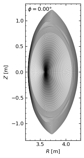
Grid lines for one zone#
Let us first instantiate the Grid class, where we automatically load the grid data.
Grid(zone='zone0', dataset='/Users/koyo/Library/Caches/cherab/lhd/emc3/grid-360.nc')
Then we plot the grid lines in the poloidal plane.
[3]:
grid.plot(linewidth=0.1)
[3]:
(<Figure size 768x576 with 1 Axes>, <Axes: xlabel='$R$ [m]', ylabel='$Z$ [m]'>)
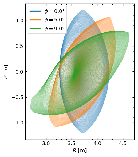
Let us plot the grid lines at several toroidal angles.
[4]:
fig, ax = plt.subplots()
n_phis = [0, 20, -1]
for i, n_phi in enumerate(n_phis):
    fig, ax = grid.plot(
        fig=fig,
        ax=ax,
        n_phi=n_phi,
        linewidth=0.1,
        color=f"C{i}",
        show_phi=False,
    )

# Add a legend
phis = grid.data_array["ζ"]
proxy = [plt.Line2D([0], [0], color=f"C{i}", lw=2) for i in range(len(n_phis))]
ax.legend(proxy, [f"$\\phi=${phi}°" for phi in phis.isel(ζ=n_phis).data]);
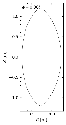
You can also plot the grid outlines in the poloidal plane.
[5]:
[5]:
(<Figure size 768x576 with 1 Axes>, <Axes: xlabel='$R$ [m]', ylabel='$Z$ [m]'>)
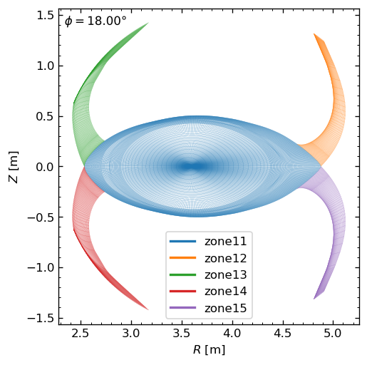
Grid lines for several zones#
EMC3-EIRENE-defined grid for LHD is divided into several zones. We can plot the grid lines with different colors for each zone.
[6]:
zones = ["zone11", "zone12", "zone13", "zone14", "zone15"]

fig, ax = plt.subplots()
show_phi = True
for i, zone in enumerate(zones):
    Grid(zone).plot(fig=fig, ax=ax, linewidth=0.1, n_phi=-1, show_phi=show_phi, color=f"C{i}")
    show_phi = False

# Add a legend
proxy = [plt.Line2D([0], [0], color=f"C{i}", lw=2) for i in range(len(zones))]
ax.legend(proxy, [f"{zone}" for zone in zones]);
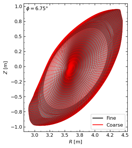
Coarse grid lines#
We define a coarse grid by selecting specific grid lines, which are intended to be used for tomography reconstruction. Here we compare the coarse grid with the original grid.
[7]:
fig, ax = plt.subplots()
grid = Grid("zone0")
grid.plot(ax=ax, linewidth=0.25, n_phi=-10)
grid.plot_coarse(ax=ax, color="red", linewidth=0.5, n_phi=-10)

# Add a legend
proxy = [plt.Line2D([], [], color=color) for color in ["black", "red"]]
ax.legend(proxy, ["Fine", "Coarse"], fontsize=10, loc="lower right");